
具体描述
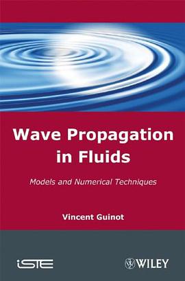
This book presents the physical principles of wave propagation in fluid mechanics and hydraulics. The mathematical techniques that allow the behavior of the waves to be analyzed are presented, along with existing numerical methods for the simulation of wave propagation. Particular attention is paid to discontinuous flows, such as steep fronts and shock waves, and their mathematical treatment. A number of practical examples are taken from various areas fluid mechanics and hydraulics, such as contaminant transport, the motion of immiscible hydrocarbons in aquifers, river flow, pipe transients and gas dynamics. Finite difference methods and finite volume methods are analyzed and applied to practical situations, with particular attention being given to their advantages and disadvantages. Application exercises are given at the end of each chapter, enabling readers to test their understanding of the subject.
作者简介
目录信息
Table of Contents......Page 7
Introduction......Page 17
1.1.1. Hyperbolic scalar conservation laws......Page 21
1.1.2. Derivation from general conservation principles......Page 23
1.1.3. Non-conservation form......Page 26
1.1.4. Characteristic form – Riemann invariants......Page 27
1.2.1. Representation in the phase space......Page 29
1.2.2. Initial conditions, boundary conditions......Page 32
1.3.1. Physical context – conservation form......Page 34
1.3.2. Characteristic form......Page 36
1.3.3. Example: movement of a contaminant in a river......Page 37
1.4.1. Physical context – conservation form......Page 41
1.4.2. Characteristic form......Page 43
1.4.3. Example: propagation of a perturbation in a fluid......Page 44
1.5.1. Physical context – conservation form......Page 48
1.5.2. Non-conservation and characteristic forms......Page 49
1.5.3. Expression of the celerity......Page 51
1.5.4. Specific case: flow in a rectangular channel......Page 54
1.5.5. Summary......Page 55
1.6.1. Physical context – conservation form......Page 56
1.6.2. Characteristic form......Page 59
1.6.3. Example: decontamination of an aquifer......Page 60
1.7.1. Physical context – conservation form......Page 62
1.7.2. Characteristic form......Page 65
1.7.3. Summary......Page 67
1.8.2.1. Exercise 1.1: the inviscid Burgers equation......Page 68
1.8.2.2. Exercise 1.2: the kinematic wave equation......Page 69
1.8.2.3. Exercise 1.3: the kinematic wave equation......Page 70
1.8.2.4. Exercise 1.4: the Buckley-Leverett equation......Page 71
1.8.2.5. Exercise 1.5: linear advection with adsorption-desorption......Page 72
2.1.1. Hyperbolic systems of conservation laws......Page 75
2.1.2. Hyperbolic systems of conservation laws – examples......Page 77
2.1.3. Characteristic form – Riemann invariants......Page 79
2.2.1. Domain of influence, domain of dependence......Page 82
2.2.2. Existence and uniqueness of solutions – initial and boundary conditions......Page 84
2.3.2. Conservation form......Page 85
2.3.3. Characteristic form......Page 88
2.3.4. Physical interpretation......Page 90
2.4.1. Physical context – hypotheses......Page 91
2.4.2.2. Continuity equation......Page 93
2.4.2.4. Simplification – vector form......Page 97
2.4.3. Characteristic form – Riemann invariants......Page 98
2.4.4.1. Treatment of internal points......Page 102
2.4.4.2. Treatment of boundary conditions......Page 104
2.4.4.3. Bergeron’s graphical method......Page 106
2.5.1. Physical context – hypotheses......Page 107
2.5.2.1. Notation......Page 108
2.5.2.2. Continuity equation......Page 109
2.5.2.3. Momentum equation......Page 110
2.5.3.1. Non-conservation form......Page 114
2.5.3.2. Characteristic form......Page 117
2.5.3.3. Expression of the speed of the waves in still water......Page 118
2.5.3.4. Riemann invariants......Page 121
2.5.4.1. The various possible flow regimes......Page 125
2.5.4.2. Treatment of internal points......Page 127
2.5.4.3. Treatment of boundary conditions......Page 129
2.5.4.4. Boundary conditions for a rectangular channel......Page 130
2.6.1. Physical context – hypotheses......Page 132
2.6.2.1. Definitions – notation......Page 134
2.6.2.2. Continuity equation......Page 135
2.6.2.3. Momentum equation......Page 136
2.6.2.4. Energy equation......Page 137
2.6.3. Characteristic form – Riemann invariants......Page 138
2.6.4.1. The various possible flow regimes......Page 142
2.6.4.2. Treatment of internal points......Page 144
2.6.4.3. Treatment of boundary points......Page 145
2.6.5. Summary......Page 146
2.7.1. What you should remember......Page 147
2.7.2.1. Exercise 2.1: the water hammer equations......Page 148
2.7.2.2. Exercise 2.2: the water hammer equations......Page 149
2.7.2.3. Exercise 2.3: the water hammer equations......Page 150
2.7.2.5. Exercise 2.5: the Saint Venant equations......Page 151
2.7.2.6. Exercise 2.6: the Saint Venant equations......Page 152
2.7.2.7. Exercise 2.7: the Euler equations......Page 153
3.1.1. Governing mechanisms......Page 155
3.1.2. Local invalidity of the characteristic formulation – graphical approach......Page 158
3.1.3.1. Free surface flow: the breaking of a wave......Page 160
3.1.3.2. Aerodynamics: supersonic flight......Page 161
3.2.1. Shock wave......Page 163
3.2.2. Rarefaction wave......Page 164
3.2.4. Mixed/compound wave......Page 165
3.3.1. Definition and properties......Page 166
3.3.2. Generalized Riemann invariants......Page 167
3.4.1. Definitions......Page 169
3.4.3. Jump relationships......Page 170
3.4.4.1. Example 1: the inviscid Burgers equation......Page 172
3.4.4.2. Example 2: the hydraulic jump......Page 174
3.4.5. The entropy condition......Page 177
3.4.6. Irreversibility......Page 179
3.4.7. Approximations for the jump relationships......Page 180
3.5.1. What you should remember......Page 181
3.5.2.2. Exercise 3.2: the kinematic wave equation......Page 182
3.5.2.4. Exercise 3.4: the Saint Venant equations......Page 183
3.5.2.5. Exercise 3.5: the Euler equations......Page 184
4.1.1. The Riemann problem......Page 185
4.1.2. The generalized Riemann problem......Page 186
4.2.1. The linear advection equation......Page 187
4.2.2. The inviscid Burgers equation......Page 188
4.2.3. The Buckley-Leverett equation......Page 190
4.3.1. General principle......Page 195
4.3.2. Application to the water hammer problem: sudden valve failure......Page 196
4.3.3.1. Introduction......Page 199
4.3.3.2. Wave pattern......Page 200
4.3.3.3. Calculation of the solution......Page 201
4.3.3.4. A specific case: dambreak on a dry bed......Page 204
4.3.4.2. Wave pattern......Page 206
4.3.4.3. Calculation of the solution......Page 209
4.4.1. What you should remember......Page 212
4.4.2.1. Exercise 4.1: the Saint Venant equations......Page 213
4.4.2.2. Exercise 4.2: the Euler equations......Page 214
5.1.1. Scalar laws......Page 215
5.1.2. Two-dimensional hyperbolic systems......Page 217
5.1.3. Three-dimensional hyperbolic systems......Page 219
5.2. Derivation from conservation principles......Page 220
5.3.1.1. The bicharacteristic approach......Page 223
5.3.1.2. The secant plane approach......Page 226
5.3.1.3. Domain of influence, domain of dependence......Page 228
5.3.2. Three-dimensional hyperbolic systems......Page 230
5.4.1.1. Physical context – hypotheses......Page 231
5.4.1.2. Continuity equation......Page 233
5.4.1.3. Equation for the momentum in the x-direction......Page 234
5.4.1.5. Vector form......Page 236
5.4.2.1. Characteristic surfaces......Page 237
5.4.2.2. Derivation of the Riemann invariants......Page 240
5.4.3.1. Domain of influence, domain of dependence......Page 242
5.4.3.2. Calculation of the solution......Page 244
5.5.2.1. Exercise 5.1: the Doppler effect......Page 245
5.5.2.2. Exercise 5.2: visual assessment of the Mach number......Page 246
6.1.1. Discretization for one-dimensional problems......Page 249
6.1.2. Multidimensional discretization......Page 250
6.1.3. Explicit schemes, implicit schemes......Page 251
6.2.1.1. Principle of the method......Page 252
6.2.1.2. Interpolation at the foot of the characteristic: first-order formula......Page 254
6.2.1.3. Interpolation at the foot of the characteristic: second-order formula......Page 258
6.2.1.4. Estimation of the source term......Page 259
6.2.1.5. Treatment of boundary conditions......Page 260
6.2.2.1. Principle of the method......Page 261
6.2.2.2. Application example: the water hammer equations......Page 263
6.2.3.1. The linear advection equation......Page 266
6.2.3.2. The inviscid Burgers equation......Page 268
6.3.1. The explicit upwind scheme (non-conservation version)......Page 270
6.3.2. The implicit upwind scheme (non-conservation version)......Page 272
6.3.3. Conservative versions of the implicit upwind scheme......Page 273
6.3.4. Application examples......Page 275
6.4.1. Formulation......Page 277
6.4.2. Estimation of nonlinear terms – algorithmic aspects......Page 280
6.4.3. Numerical applications......Page 281
6.5.1. The Crank-Nicholson scheme......Page 287
6.5.2. Centered schemes with Runge-Kutta time stepping......Page 288
6.6.1. Definitions......Page 290
6.6.2. General formulation of TVD schemes......Page 291
6.6.3. Harten’s and Sweby’s criteria......Page 294
6.6.4. Traditional limiters......Page 296
6.6.5. Calculation example......Page 297
6.7.1. Principle of the approach......Page 300
6.7.2.1. Explicit upwind scheme for the water hammer equations......Page 303
6.7.2.2. TVD scheme for the water hammer equations......Page 305
6.7.2.3. Calculation example......Page 307
6.8.1. Motivation and principle of the approach......Page 309
6.8.2.1. Roe’s method......Page 310
6.8.2.2. Expression in the base of eigenvectors......Page 312
6.9.1. Explicit alternate directions......Page 313
6.9.2. The ADI method......Page 316
6.9.3. Multidimensional schemes......Page 318
6.10.1. What you should remember......Page 319
6.10.2.3. Exercise 6.3: finite difference methods for hyperbolic systems......Page 321
7.1.1. One-dimensional conservation laws......Page 323
7.1.2. Multidimensional conservation laws......Page 325
7.1.3. Application to the two-dimensional shallow water equations......Page 328
7.2.1. Principle......Page 330
7.2.2.1. Discretization......Page 331
7.2.2.2. Flux calculation at internal interfaces......Page 332
7.2.2.3. Boundary conditions......Page 333
7.2.2.4. Calculation of the liquid discharge at the cell interfaces......Page 334
7.2.2.5. Algorithm......Page 335
7.2.3.2. Flux calculation at internal interfaces......Page 336
7.2.3.3. Boundary conditions......Page 338
7.2.4.1. Discretization......Page 339
7.2.4.2. Flux calculation at internal interfaces......Page 341
7.2.4.3. Treatment of boundary conditions......Page 342
7.3.1.1. Historical perspective......Page 344
7.3.1.2. Reconstruction of the flow variable......Page 345
7.3.1.3. Slope limiting......Page 346
7.3.1.5. Flux calculation and balance......Page 347
7.3.2.2. Slope limiting......Page 348
7.3.2.3. Solution of the generalized Riemann problem......Page 349
7.4.1. What you should remember......Page 350
7.4.2. Suggested exercises......Page 351
A.1. Definitions......Page 353
A.2.2. Multiplication by a scalar......Page 355
A.2.4. Determinant of a matrix......Page 356
A.3.1. Differentiation......Page 357
A.4.1. Definitions......Page 358
A.4.2. Example......Page 359
B.1.2. Principle of a consistency analysis......Page 361
B.1.3. Numerical diffusion, numerical dispersion......Page 363
B.2.1. Definition......Page 365
B.2.2. Principle of a stability analysis......Page 366
B.2.3.1. The linear advection equation......Page 368
B.2.3.2. The diffusion equation......Page 369
B.2.3.3. The advection-dispersion equation......Page 371
B.2.4. Harmonic analysis of numerical solutions......Page 372
B.2.5. Amplitude and phase portraits......Page 375
B.2.6. Extension to systems of equations......Page 377
B.3.2. Lax’s theorem......Page 379
C.1.1. HLL solver......Page 381
C.1.2. HLLC solver......Page 383
C.2. Roe’s solver......Page 386
Appendix D. Summary of the Formulae......Page 389
References......Page 395
Index......Page 399
· · · · · · (收起)
读后感
用户评价
这本书的封面设计倒是挺有意思,深邃的蓝色调,让人联想到广阔无垠的海洋或者高空的宁静。我刚拿到手的时候,心里是充满期待的,毕竟“流体中的波的传播”这个主题听起来就充满了物理学的魅力。然而,当我翻开第一页,试图寻找那些熟悉的数学公式和严谨的理论推导时,却发现内容似乎有些……跑偏了?它更像是一本关于“声学在不同介质中如何影响人类感知”的哲学探讨,而非我所期望的那种硬核的物理教材。作者花费了大量的篇幅去描述声音在水下环境中的历史演变,比如早期潜艇声呐的局限性,以及艺术作品中如何运用声波来营造特定的情绪氛围。我对这种侧重于人文和历史的叙述方式感到有些困惑,因为我对理解波动方程的具体解法更感兴趣。书中的插图也多是抽象的艺术构图,而不是清晰的物理模型示意图。这使得阅读过程充满了意外,每翻一页都在猜测作者接下来会探讨哪种完全不相关的领域。说实话,如果你想找一本能帮你搞定期末考试的专业书籍,这本书可能不是最佳选择,但如果你对声音的文化意义和历史足迹感兴趣,或许能从中找到一些新奇的视角。整体来看,它更像是一本介于科学随笔和文化评论之间的作品,远没有标题所暗示的那种精确性与深度。
这本书的语言风格极其晦涩,充满了老派的学术腔调,读起来令人感到一种沉重的、几乎是巴洛克式的复杂性。作者似乎有一种强烈的倾向,即用尽可能多的从句和复杂的长句来表达一个原本可以用简单陈述句概括的物理概念。例如,在讨论瑞利-泰勒不稳定性时,一个本应清晰描述的界面失稳过程,被包装成了一段长达八行的、充满了过去分词和状语从句的文字迷宫。我必须逐字逐句地拆解句子结构,才能勉强抓住其背后的物理图像。更令人沮丧的是,作者经常使用一些非常生僻的、几乎已被现代物理学界淘汰的术语来指代现代常用的概念。我不得不频繁地查阅注释,试图去对应“涡旋密度梯度张量”这种令人头晕的表达与我们今天所说的“旋度”之间的关系。这种对语言的“过度修饰”,极大地阻碍了知识的有效传递。阅读此书,与其说是学习知识,不如说是在进行一场艰苦的语言破译工作。如果作者的目标是让更多人理解流体中的波现象,那么他无疑选择了最反直觉的方式来实现这一目标。它更像是为那些早已精通该领域、并乐于欣赏古典学术文风的学者所作,对于新手而言,简直是知识的“防火墙”。
我原本寄希望于这本书能提供关于超声波在生物组织中应用的一些最新进展,特别是关于聚焦超声消融术中能量衰减和波前畸变的数值模拟方法。然而,这本书的内容止步于上世纪六十年代的经典理论框架,甚至连对傅里叶变换在时域分析中的标准应用都没有给出清晰的步骤演示。书中对“波动”的理解似乎停留在非常宏观的、偏向于流体力学的角度,完全忽略了微观粒子相互作用对波速和衰减率的精细影响。当涉及到数值方法时,作者仅仅泛泛地提到了有限差分法的概念,却没有提供任何关于网格划分、边界条件处理,或者如何选择合适的离散化格式来保证非线性问题的稳定性的具体指导。对于一个热衷于计算物理的读者来说,这简直是信息真空。它像是一本厚厚的、用优美的散文诗形式写成的“物理学散步指南”,而不是一本用于解决实际问题的工具书。它详述了波的形态和历史,却对如何用现代工具去量化和预测这些形态变化讳莫如深。如果要用一句话概括我的感受,那就是:它给了我一篇精彩的关于“河流”的文学描述,却完全没有教我如何建造一座跨越河流的桥梁。
这本书的排版简直是一场视觉上的灾难,我甚至怀疑排版人员是不是和作者有什么深仇大恨。纸张的质量倒是过得去,拿在手里有一定的分量感,但这并不能掩盖内文排版上的诸多问题。字体选择上,作者似乎偏爱一种细长、略带花哨的衬线体,在处理大段落的数学公式时,那些复杂的希腊字母和上下标挤在一起,简直是令人抓狂的“视觉噪声”。我不得不反复对照公式手册才能确认某个符号到底代表什么。更要命的是,图表的缺失和位置的错位。某些关键的能量守恒图示,被硬生生地切在了页面的边缘,或者干脆被安排在了十页之后,完全打断了逻辑的连贯性。我阅读物理类书籍的习惯是从图例入手理解概念,但这本书的配图少得可怜,寥寥几张也模糊不清,仿佛是上世纪八十年代的低分辨率扫描件。我试着去理解那些关于流体动力学稳定性的章节,但因为缺乏直观的图形辅助,那些复杂的边界条件描述读起来就像是绕口令。我花了大量时间去“重建”作者心中本应存在的图示,这大大降低了阅读效率和乐趣。一本关于“传播”的书,其自身的结构和信息传播方式却如此滞涩晦涩,实在是一种莫大的讽刺。
我买这本书的初衷,是希望深入理解非线性声学效应在复杂流体介质中是如何建模和求解的。我期待的是对纳维-斯托克斯方程进行适当简化后,如何引入非线性项来描述空化现象或冲击波的形成。然而,这本书似乎完全避开了这些核心的、具有挑战性的数学物理问题。相反,它花了好几章的篇幅,详细描述了二十世纪初关于声波在水下导航中的“误解与发现”,着重于那些已经被现代技术完全取代的早期实验方法。其中对特定历史人物的生平事迹的侧写,占用了过多篇幅,这些内容对于一个寻求前沿理论指导的读者来说,显得既冗余又无关痛痒。比如,作者用了整整一章来分析一位早期科学家如何因为设备简陋而错误地测量了某个特定频率下的传播速度,并花费了大量笔墨来赞扬他的“探索精神”。这种叙事方式,与其说是在探讨物理现象,不如说是在进行一场缓慢而温情的历史回顾。我需要的是“如何计算”,而不是“谁在什么时候搞错了什么”。如果说这本书有什么价值,那就是它提供了一个非常详尽的、关于声学研究史的“轶事集锦”,但它在提供任何有用的、可应用于工程实践的数学工具方面,几乎是完全失职的。